From Raw to Ready: Rapid Sentinel-2 Index Workflows for Time-Sensitive Use Cases
Field notes on rebuilding cloud-optimized index coverage under a deadline. When processed NDVI and LAI data disappears days before it is due, a cloud-native pipeline turns the crisis into a batch job. Story, architecture, code, and the lessons that held up under pressure.
ELEMNT Engineering· ~15 min read
Every team that works with satellite imagery has a version of this nightmare. The derived data, the part you actually serve, is gone. The raw archive is safe in cold storage, but the expensive part vanished: the processed indexes, the cloud-masked composites, the catalog that made any of it findable. And the deadline did not move.
This post walks through one such recovery, told as an engineering scenario. The figures are illustrative, but the architecture and the code are real, reusable patterns. The point is not the panic. The point is that a cloud-native design makes the panic boring.
Four days before the deadline
The trigger was mundane: the object store holding processed results failed. With it went roughly 25,000 Sentinel-2 scenes' worth of processed imagery, and the NDVI and LAI indexes derived from them, about 50,000 derived assets in all. There was no backup. The clock read four days until the data was due for an environmental monitoring program that depended on it.
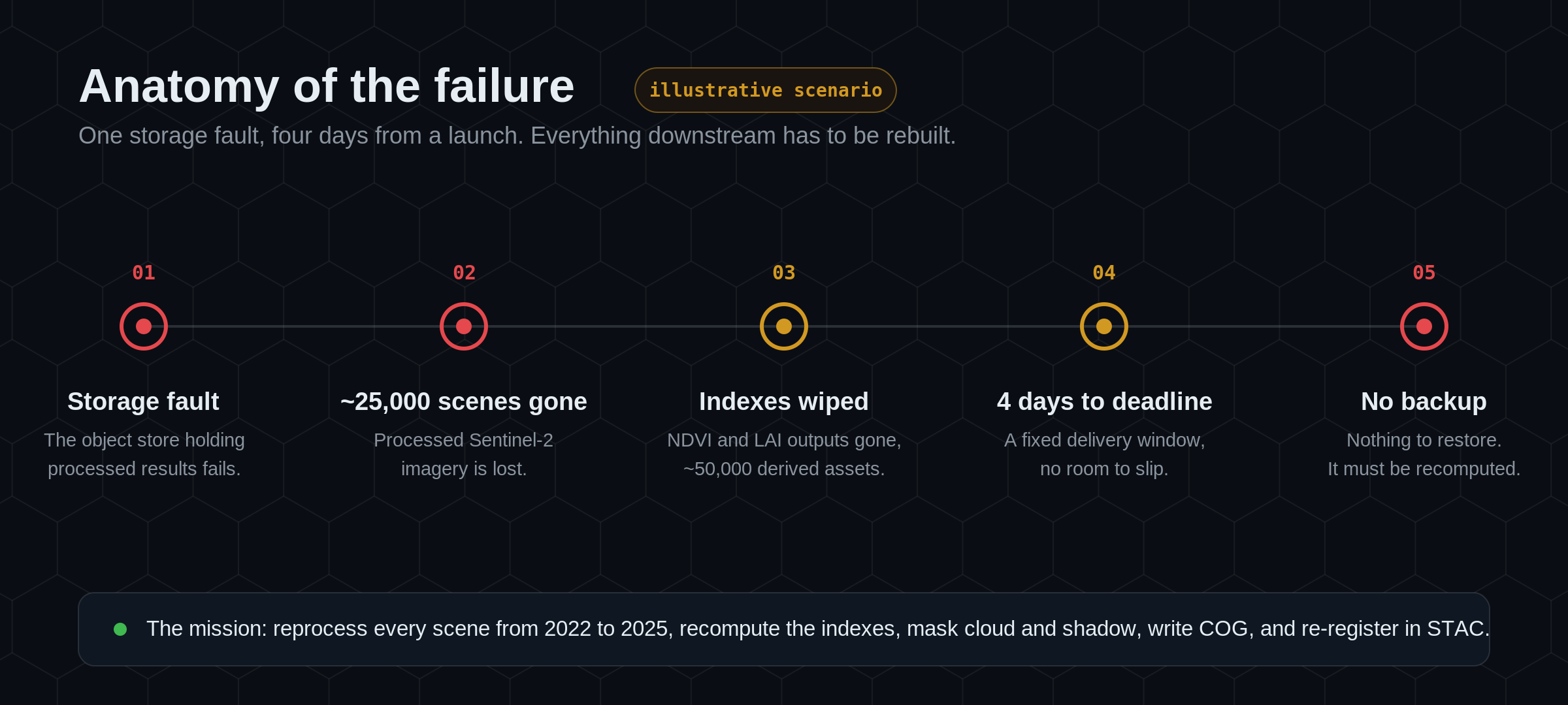
One detail saved the week: the raw Sentinel-2 Level-2A archive was intact. That is the whole strategy in a sentence. If you can reprocess deterministically from raw inputs, lost derivatives are not a catastrophe. They are a queue.
The mission
The work was clear, if large. Reprocess every Sentinel-2 scene from 2022 to 2025. For each scene: recompute NDVI and LAI, mask out cloud, cirrus, and shadow, convert every output to Cloud-Optimized GeoTIFF, and re-register the lot in a STAC catalog so applications could find it again. Do it in four days, on whatever compute could be rented for the window.
The instinct in a moment like this is to reach for a bigger machine. The better answer is to reach for more small ones, and to make the work splittable enough that they can all run at once.
The tiling grid is the unit of work
Sentinel-2 ships on a fixed global tiling scheme, the Military Grid Reference System (MGRS), with 100 km tiles, each carrying a stable ID. That fixed grid is the gift. Every tile is an independent, re-runnable unit, so recovery stops being one enormous job and becomes a queue of thousands of small, identical ones, each scoped to a single tile and date.
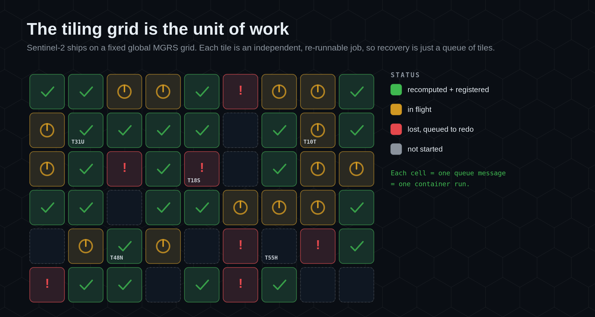
Because tile IDs are deterministic, you can diff what should exist against what does, produce the exact list of missing tile and date combinations, and push that straight onto a queue. The lost data effectively becomes a worklist, and a worklist is something a fleet of workers can chew through in parallel.
Six principles that make it boring
None of the ideas below are new. Stacked together, they are what turns a data-loss emergency into a routine bulk run.
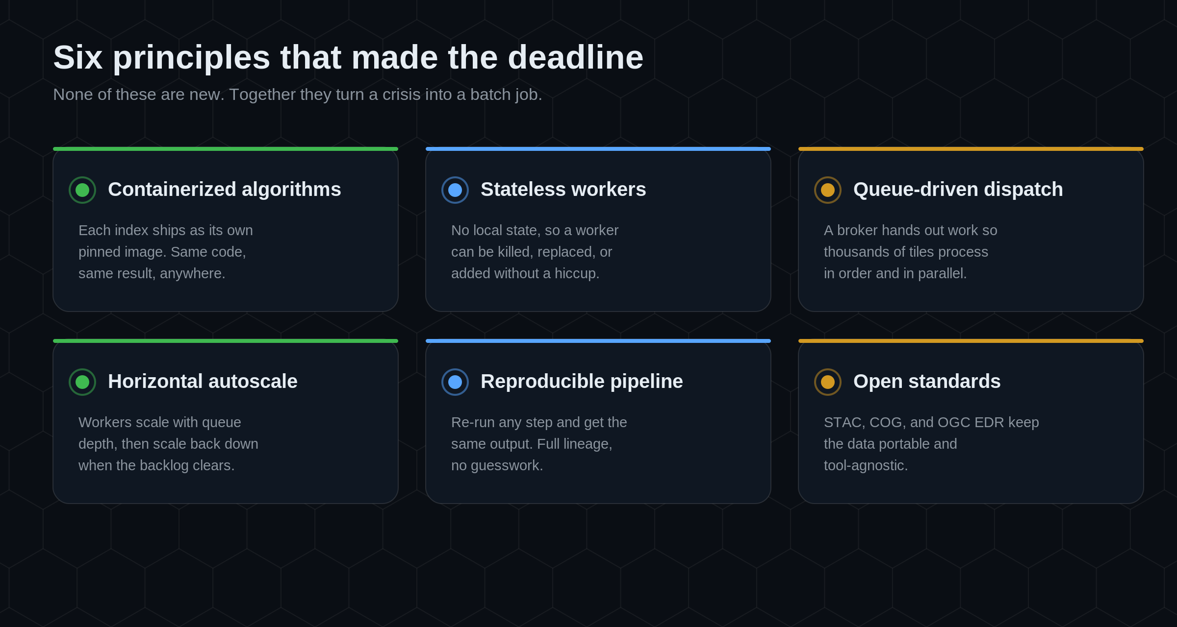
Each index algorithm ships as its own container, pinned to a version, so the same code produces the same result on any node. The workers that run them are stateless: they hold no local state, so any worker can be killed, replaced, or added without disrupting the run. Work is handed out through a queue, which keeps thousands of tiles processing in order and in parallel. The fleet autoscales horizontally with queue depth, then scales back down when the backlog clears. The pipeline is reproducible, so re-running any step yields the same output with full lineage. And every artifact lands in an open standard, which is what keeps the result portable once the dust settles.
The pipeline
Here is how those principles fit together end to end.
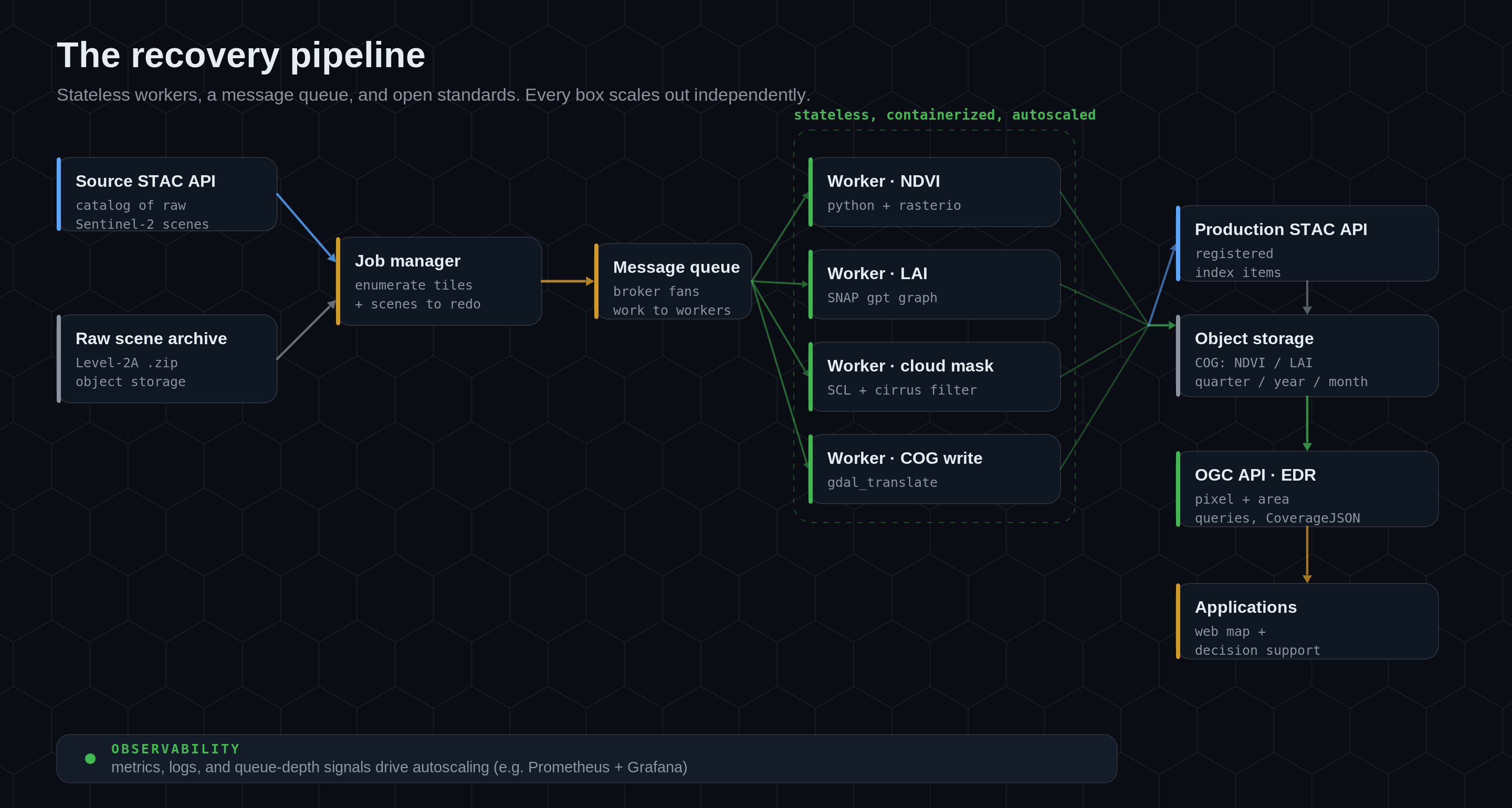
A source STAC API describes the raw scenes, and the raw archive holds the Level-2A products in object storage. A job manager enumerates the missing tiles and pushes one message per tile onto a message queue. The broker fans that work out to a pool of stateless, containerized workers: one image computes NDVI with Python and rasterio, another runs the LAI biophysical processor, others handle cloud masking and COG conversion. As each tile finishes, results are written to object storage as COG and registered in a production STAC API. On top of that sits an OGC API EDR endpoint for pixel and area queries, which is what the applications actually call. Underneath everything, observability (metrics, logs, and queue-depth signals) drives the autoscaling decisions.
Nothing in that diagram is exotic. That is the point. Each box scales out on its own, and no box has to know how many of any other box exist.
The processing code
The two indexes are computed by two small, self-contained workers. NDVI is the simpler of the pair: two bands, one ratio.
import glob, zipfile
import numpy as np
import rasterio

# 1. Unpack the raw Level-2A products for this tile.
for path in glob.glob("storage/sentinel-2/*.zip"):
    with zipfile.ZipFile(path, "r") as zf:
        zf.extractall("storage")

# 2. Find the two 10 m bands NDVI needs: B04 (red) and B08 (NIR).
bands = glob.glob("storage/**/IMG_DATA/**/*.jp2", recursive=True)
red_path = next(p for p in bands if "B04_10m" in p)
nir_path = next(p for p in bands if "B08_10m" in p)

with rasterio.open(red_path) as red_src:
    red = red_src.read(1).astype("float32")
    profile = red_src.profile
with rasterio.open(nir_path) as nir_src:
    nir = nir_src.read(1).astype("float32")

# 3. NDVI = (NIR - RED) / (NIR + RED), guarding the divide-by-zero.
denominator = nir + red
ndvi = np.where(denominator == 0, np.nan, (nir - red) / denominator)

# 4. Write a float32 GeoTIFF, ready to be cloud-optimized next.
profile.update(driver="GTiff", dtype="float32", count=1)
with rasterio.open("ndvi.tif", "w", **profile) as dst:
    dst.write(ndvi.astype("float32"), 1)
Two facts make this reliable at scale. The bands are addressed by name (B04_10m, B08_10m), not by position, so the worker does not care how the archive is laid out. And invalid pixels are set to NaN rather than zero, so a cloudless ratio is never confused with a no-data hole when the cloud mask is applied downstream.
LAI is heavier. It runs through the SNAP biophysical processor, driven by a graph file, so the worker's job is to point a known-good graph at this scene and run it.
import glob, subprocess, resource
import xml.etree.ElementTree as ET

# 1. Load a SNAP processing graph for the LAI biophysical processor.
graph_path = glob.glob("snap_graphs/*/graph.xml")[0]
tree = ET.parse(graph_path)
root = tree.getroot()

# 2. Point the graph at this scene's input and the desired output.
input_product = glob.glob("storage/*/MTD*.xml")[0]
lai_output = "storage/lai.tif"
for index, node in enumerate(root.iter("file")):
    node.text = input_product if index == 0 else lai_output

tree.write("storage/graph_resolved.xml", xml_declaration=True, encoding="utf-8")

# 3. Run SNAP's graph processing tool, giving it room to breathe.
resource.setrlimit(resource.RLIMIT_AS,
                   (resource.RLIM_INFINITY, resource.RLIM_INFINITY))
subprocess.run(
    ["/usr/local/snap/bin/gpt", "-J-Xmx16g", "-q", "4",
     "storage/graph_resolved.xml"],
    check=True,
)
The shape is the same as NDVI: take a tile, produce a single-band float raster, move on. Because both workers are stateless and containerized, the only difference the queue sees is that an LAI job holds a node for longer. Autoscaling absorbs that difference without anyone tuning it by hand.
Cloud-optimize, catalog, serve
Computing the index is half the job. The other half is making it cheap to find and cheap to read, which is entirely a matter of format and catalog.
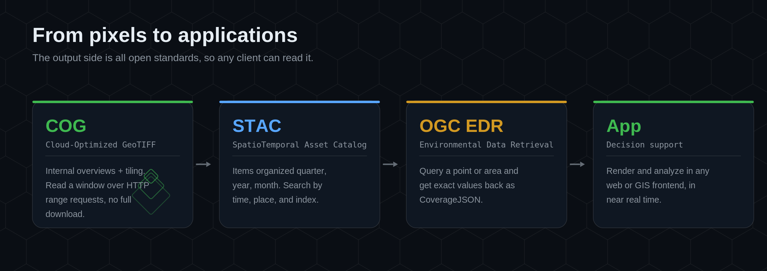
Every output is converted to COG, a GeoTIFF with internal overviews and tiling, so a client can read a small window over HTTP range requests instead of downloading the whole file. Each COG is registered as an item in a STAC catalog, organized by quarter, year, and month, which makes the archive searchable by time, place, and index. On top of the catalog, OGC API EDR answers the question applications actually ask: give me the value at this point, or across this area, and hand it back as CoverageJSON. The result renders in any web or GIS frontend, in near real time, with no bespoke tile server in the path.
This is the part worth internalizing. Because the output side is all open standards, the recovered data is not locked to the pipeline that produced it. Any STAC client can browse it, any COG reader can open it, and any EDR client can query it.
A real use case: crop health in a narrow window
The reason any of this had a deadline is agronomic. Consider an agriculture team monitoring crop health across a growing region [illustrative scenario, pre-GA model]. NDVI, queried per field through EDR, tracks plant vigor over the season and flags fields that are lagging. LAI, the leaf area index, feeds a fertilizer recommendation so that rice gets the right input at the right growth stage. Both decisions live inside a narrow seasonal window. A week late is not a smaller insight, it is no insight, because the window has closed.
That is what "time-sensitive" means in practice. The value of the index is not just its accuracy. It is whether it arrives while the decision is still open. A recovery pipeline that can rebuild a multi-year archive in days is really a pipeline that can keep a seasonal decision on schedule.
Lessons learned
Four things held up under pressure, and they are the parts worth copying.
Workload and performance. Sizing the fleet to queue depth, not to a guess, is what kept the run inside four days. Heavy jobs (LAI) and light jobs (NDVI) share the same queue, and horizontal scaling, not a bigger box, closes the gap.
Data management. Treating raw inputs as the source of truth and every derivative as reproducible output is the decision that made recovery possible at all. The deterministic tile grid turned "what did we lose" into a query rather than an investigation.
Distribution. Committing to open formats up front (COG, STAC, OGC EDR) meant the rebuilt data was immediately usable by every downstream client, with nothing to re-integrate.
Monitoring. Metrics and dashboards were not a nice-to-have during the run, they were the steering wheel. Queue depth, worker health, and throughput are what told the team whether four days was actually enough, early enough to add capacity.
Why it worked
Recovery succeeded because the architecture was already built on open standards, containerization, statelessness, and reproducibility. Open standards made the output portable. Modularity let each step iterate independently. Containers gave consistent execution across whatever compute was available. Reproducible pipelines guaranteed that re-running a lost tile produced exactly the right result. And cloud-native scaling meant the whole fleet could grow to meet the deadline and shrink the moment it passed. The crisis did not call for heroics. It called for a queue and enough workers.
Where ELEMNT fits
Everything above is open tooling and open standards, and that is deliberate. ELEMNT is the cloud-native geospatial data platform built around exactly this shape: a STAC catalog for discovery, a message-driven compute tier for processing, object storage for COG and other open formats, and OGC-standards-aligned access on top. PMTiles, COG, GeoParquet, and Zarr are served straight from object storage behind a global edge, so there is no tile server in the path and the per-tile serving cost works out to about $0.0000141 per tile on ELEMNT's published architecture.¹
The same properties that make a recovery boring make day-to-day work cheaper. Bring your own datastore, keep your data in open formats, self-host any time, and pay only for what you use, with no bill shock when a seasonal job spikes the queue. The honest caveat: ELEMNT's Git-style versioning lands in Q4 2026 and real-time collaboration in Q1 2027, so the lineage story above is, for now, something you assemble from reproducible pipelines and STAC, not a single in-platform "undo."
This is presented as an illustrative engineering walkthrough. The recovery figures (≈25,000 scenes, ≈50,000 assets, four days) are scenario parameters, not a customer-reported result. The architecture and code are real, reusable patterns. ELEMNT is pre-launch.
¹ Per-tile serving cost is ELEMNT's published architecture figure (≈$0.0000141/tile at 50M tiles/month), not a customer-reported result.
Technical references: Sentinel-2 MGRS tiling and Level-2A products (Copernicus / ESA), the Scene Classification Layer for cloud and cirrus masking, the SNAP biophysical (LAI) processor, and the open standards STAC, Cloud-Optimized GeoTIFF, and OGC API EDR (CoverageJSON).
What is ELEMNT?
ELEMNT is the cloud-native geospatial data platform — open formats (PMTiles, COG, Zarr, GeoParquet) served straight from object storage, OGC API-compliant, with transparent pay-per-use pricing and no vendor lock-in. From a single project to a billion tiles. Earth Traffic is one demo of what it can do.